Email me: mjcaywt@gmail.com
2015年9月10日星期四
2014年4月4日星期五
Week11:Sorting and Efficiency
In this week, we talked about a lot of sorting and its efficiency, such as merge_sort, quick_sort and tim-sort(Python's built-in sort).
Most sorting algorithms work by comparing the data being sorted. In some cases, it may be desirable to sort a large chunk of data (for instance, a struct containing a name and address) based on only a portion of that data. The piece of data actually used to determine the sorted order is called the key.
Sorting algorithms are usually judged by their efficiency. In this case, efficiency refers to the algorithmic efficiency as the size of the input grows large and is generally based on the number of elements to sort. Most of the algorithms in use have an algorithmic efficiency of either O(n^2) or O(n*log(n)). A few special case algorithms can sort certain data sets faster than O(n*log(n)). These algorithms are not based on comparing the items being sorted and rely on tricks. It has been shown that no key-comparison algorithm can perform better than O(n*log(n)).
Sorting algorithms are usually judged by their efficiency. In this case, efficiency refers to the algorithmic efficiency as the size of the input grows large and is generally based on the number of elements to sort. Most of the algorithms in use have an algorithmic efficiency of either O(n^2) or O(n*log(n)). A few special case algorithms can sort certain data sets faster than O(n*log(n)). These algorithms are not based on comparing the items being sorted and rely on tricks. It has been shown that no key-comparison algorithm can perform better than O(n*log(n)).
Many algorithms that have the same efficiency do not have the same speed on the same input. Algorithms must be judged based on their average case, best case, and worst case efficiency. Some algorithms, such as quick sort, perform exceptionally well for some inputs, but horribly for others. Other algorithms, such as merge sort, are unaffected by the order of input data. Even a modified version of bubble sort can finish in O(n) for the most favorable inputs.
Here are examples of merge_sort and quick_sort that Danny provided:
"def quick(L):
    if len(L) > 1:
        pivot = L[0] # there are much better ways of choosing the pivot!
        smaller_than_pivot = [x for x in L[1:] if x < pivot]
        larger_than_pivot = [x for x in L[1:] if x >= pivot]
        return quick(smaller_than_pivot) + [pivot] + quick(larger_than_pivot)
    else:
        return L


def merge2(L1:list, L2:list) -> list:
    """return merge of L1 and L2
    NOTE: modifies L1 and L2

    >>> merge2([1, 3, 5], [2, 4, 6])
    [1, 2, 3, 4, 5, 6]
    >>> merge2([1, 2, 3], [0, 4, 5])
    [0, 1, 2, 3, 4, 5]
    >>> merge2([0], [1, 2, 3, 4])
    [0, 1, 2, 3, 4]
    """
    L = []
    L1.reverse()
    L2.reverse()
    while L1 and L2:
        if L1[-1] < L2[-1]:
            L.append(L1.pop())
        else:
            L.append(L2.pop())
    L1.reverse()
    L2.reverse()
    return L + L1 + L2


def merge(L1:list, L2:list) -> list:
    """return merge of L1 and L2
    NOTE: modifies L1 and L2

    >>> merge([1, 3, 5], [2, 4, 6])
    [1, 2, 3, 4, 5, 6]
    >>> merge([1, 2, 3], [0, 4, 5])
    [0, 1, 2, 3, 4, 5]
    >>> merge([0], [1, 2, 3, 4])
    [0, 1, 2, 3, 4]
    """
    decreasing_from_largest = []
    while L1 and L2:
        if L1[-1] > L2[-1]:
            decreasing_from_largest.append(L1.pop())
        else:
            decreasing_from_largest.append(L2.pop())
    decreasing_from_largest.reverse()
    return L1 + L2 + decreasing_from_largest


def merge_sort(L):
    """Produce copy of L in non-decreasing order

    >>> merge_sort([1, 5, 3, 4, 2])
    [1, 2, 3, 4, 5]
    """
    if len(L) < 2 :
        return L
    else :
        left_sublist = L[:len(L)//2]
        right_sublist = L[len(L)//2:]
        return merge2(merge_sort(left_sublist),
                      merge_sort(right_sublist))"
| Time | |||||||
|---|---|---|---|---|---|---|---|
| Sort | Average | Best | Worst | Space | Stability | Remarks | |
| Merge Sort | O(n*log(n)) | O(n*log(n)) | O(n*log(n)) | Depends | Stable | On arrays, merge sort requires O(n) space; on linked lists, merge sort requires constant space | |
| Quicksort | O(n*log(n)) | O(n*log(n)) | O(n^2) | Constant | Stable | Randomly picking a pivot value (or shuffling the array prior to sorting) can help avoid worst case scenarios such as a perfectly sorted array. | |
Week9
This week's focus was on binary search trees and time complexity; such as run time analysis and big o notation.
First off a binary search tree is binary tree that has a left subtree of nodes that contains values less than the value of the node while the right subtree consists of a node greater than the value of the node. I find its a very applicable model because it accounts for much faster searches. There were many instances of BST's which we've encountered such as nested lists. The useful aspect of a BST seems to be that as opposed to iterating and finding the midpoint of list, the BST begins at the midpoint and the algorithm is based on either traversing right or left. I don't see much of a difference in implementing a BST as opposed to sorting a list, perhaps when referring to larger values it may be apparent that one has better performance.
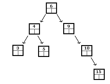
BSTs seem to also attribute qualities similar to precedent methods as insertion, sorting, searching and delete. The following is an example of a BST:

The task of sorting consists of taking data and arranging it in some sort of predetermined order. Searching consists of trying to find a particular piece of data from the total set of data. As one might expect, searching is easier once the data have been sorted.
First off a binary search tree is binary tree that has a left subtree of nodes that contains values less than the value of the node while the right subtree consists of a node greater than the value of the node. I find its a very applicable model because it accounts for much faster searches. There were many instances of BST's which we've encountered such as nested lists. The useful aspect of a BST seems to be that as opposed to iterating and finding the midpoint of list, the BST begins at the midpoint and the algorithm is based on either traversing right or left. I don't see much of a difference in implementing a BST as opposed to sorting a list, perhaps when referring to larger values it may be apparent that one has better performance.
BSTs seem to also attribute qualities similar to precedent methods as insertion, sorting, searching and delete. The following is an example of a BST:

The task of sorting consists of taking data and arranging it in some sort of predetermined order. Searching consists of trying to find a particular piece of data from the total set of data. As one might expect, searching is easier once the data have been sorted.
Week8
This week marked the introduction of linked lists, a concept which I initially imagined to be a complex archetype, however after gaining much insight it seems a much less simpler concept to apprehend.
From my understanding a linked list is quintessentially a sequence of nodes which contain values that point to another sequence or nodes. If it is not pointing to anything the value itself must be pointing to none. Danny expressed this in the lecture as classes which contained a items and values attributing to another item or value or node. A linked list is compromised of nodes as an attribute whilst referencing another node. I find the representation of linked list as a makes it the most clear. Another way of looking at it is like cargo, in a factory where each package is pointing to another package.
We covered some new methods as __len__, __contains__, __repr__, and __getitem__which I found was fairly straightforward except at first it was unclear to me what the difference between the __repr__ and __str__ method were, however after viewing some videos on youtube, it seems that __repr__ is a more formal representation of the object that can be accessed.
I found this week to be much more laid back in comparison with the previous however, the challenge was more reflected towards the understanding as opposed to application. Overall I look forward to going much more in depth with linked lists.
Week7:Recursion
This week marked the introduction to one of the central ideas to computer science; recursion. Although it was discussed briefly in the previous week, Danny went into to much more detail. The concept of recursion is somewhat straightforward in terms of human intuition as it follows the basic algorithm of a base case and repeating ideologies. The method in which recursion was performed in lecture was rather unusual in comparison to what I am familiar with; the way it was performed was as if the programmer was communicating in plain English. It seems appropriate to follow a majority of mathematical sequencing via repetition.
The notion of how to choose test cases was also discussed in reference to the exercise. Furthermore I began the challenging journey of the assignment. A mere task to create a program that reiterates the tour of hanoi problem. I found this a rather challenging task for an assignment in an introductory course to computer science as it focused mainly on recursion.
The notion of how to choose test cases was also discussed in reference to the exercise. Furthermore I began the challenging journey of the assignment. A mere task to create a program that reiterates the tour of hanoi problem. I found this a rather challenging task for an assignment in an introductory course to computer science as it focused mainly on recursion.
订阅:
博文 (Atom)